Scaling Laws for Behavioral Foundation Models
How to spend compute when you train on what people do, not what they say

Over the past few years, a quiet shift has happened inside many of the world's largest retailers, banks, and payment networks. Instead of building a separate model for every task, they have started training a single foundation model on sequences of human actions: what people search, click, buy, and tap. These behavioral foundation models are big enough that mistakes are expensive—but unlike language models, nobody had written down how to size them. This post is that missing manual. We share what we learned calibrating the four most important knobs, and a surprising conclusion: the metric you measure is part of the scaling law itself.

It builds from the ground up: the early sections explain the ideas in plain language, and the later sections turn them into a concrete recipe—specific numbers for embedder size, batch size, and the rest—aimed at teams who are actually training one of these models. If you just want the intuition, the first half stands on its own.

In 2020 and 2022, two famous results—Kaplan et al. and the Chinchilla paper—changed how language models are built. They turned a messy art ("just make it bigger?") into a clean allocation problem: given a fixed compute budget, how many parameters should you train on how many tokens? The famous Chinchilla answer is roughly 20 tokens of data per parameter. That single number has guided billions of dollars of training.

Behavioral foundation models are now everywhere in industry—at Visa, Stripe, Netflix, J.P. Morgan, and in our own BehaviorGPT line—but they have had no equivalent guidance. And they differ from language models in a way that matters a lot for scaling.

Because of this, modern behavioral systems use a two-part architecture, and that is the object we study throughout this post:

1. The event embedder. A small feature-based model that turns each raw item (its text, category, price, etc.) into a single vector. Think of it as the "translator" that gives every product a meaning.
2. The contextualizer. A decoder-only transformer—just like a GPT—that reads the sequence of event vectors and predicts the next event. Think of it as the "reader" that understands the story of a user's behavior.

This split is necessary at serving time: a real catalogue can have a hundred million items, and re-encoding all of them on every prediction is hopeless. So the deployed recipe trains in two stages—first train the embedder and contextualizer together, then freeze the embedder, cache its vectors, and keep training the contextualizer against a much larger pool of candidates. That gives us four coupled knobs to calibrate, and a fifth question hanging over all of them.

We answered these on one model stack and one real-world retail corpus—anonymized searches, views, clicks, and purchases—across roughly 600 training runs spanning four orders of magnitude of compute (\(10^{15}\) to \(10^{19}\) FLOPs). Here is what we found.

The first question is the most architectural: at a fixed compute budget, how much of your model should be the embedder versus the transformer? It would be reasonable to guess "a lot"—after all, the embedder has to understand every product in the catalogue.

The data says the opposite. We swept the embedder's share of parameters from essentially 0% all the way to 50%, at four different compute budgets. The best share is remarkably stable and surprisingly small: about 2% of parameters, at every budget we tested ().

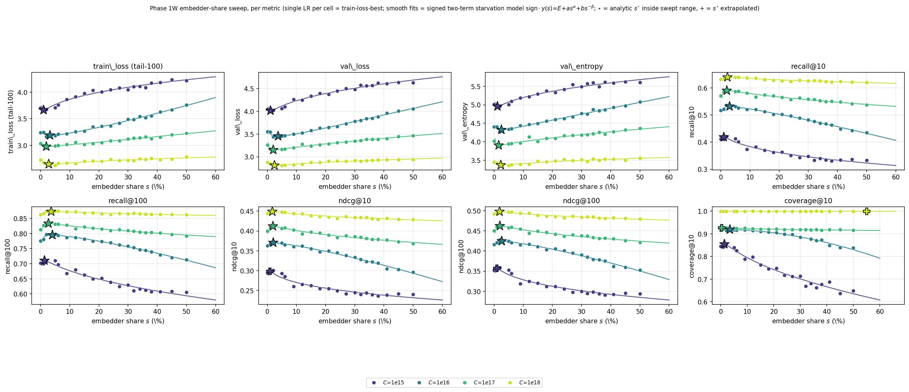
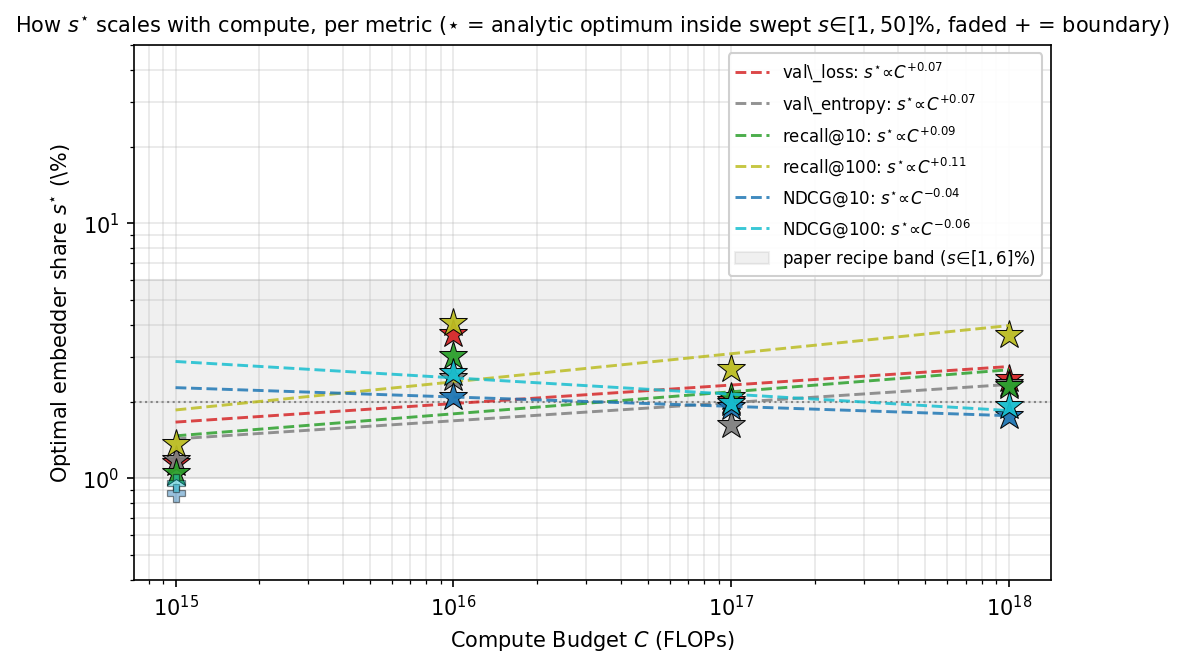
Plotting that optimum against compute makes the flatness obvious: even when we scale training compute 10,000×, the same embedder wins on the same share of fields (). This isn't a fluke of our dataset—there's a clean mechanism behind it. Two asymmetries push the embedder to stay small:

1. It's more expensive per parameter. The transformer runs once per sequence, but the embedder runs on every event in every sequence—dozens of times more often. Each embedder parameter therefore costs far more compute per step than each transformer parameter.
2. It sees the same things over and over. The transformer almost never sees the same 256-event window twice. But the embedder sees popular items—say, milk—hundreds or thousands of times. A big embedder under this repetitive diet starts to memorize rather than generalize.

In other words: the embedder is the expensive, easily-overfit part, so the compute-optimal move is to keep it lean and pour your parameters into the transformer that actually reads the behavioral story. (Fun aside: this echoes multimodal models like LLaVA and Flamingo, where a comparatively small vision encoder feeds a much larger language model.)

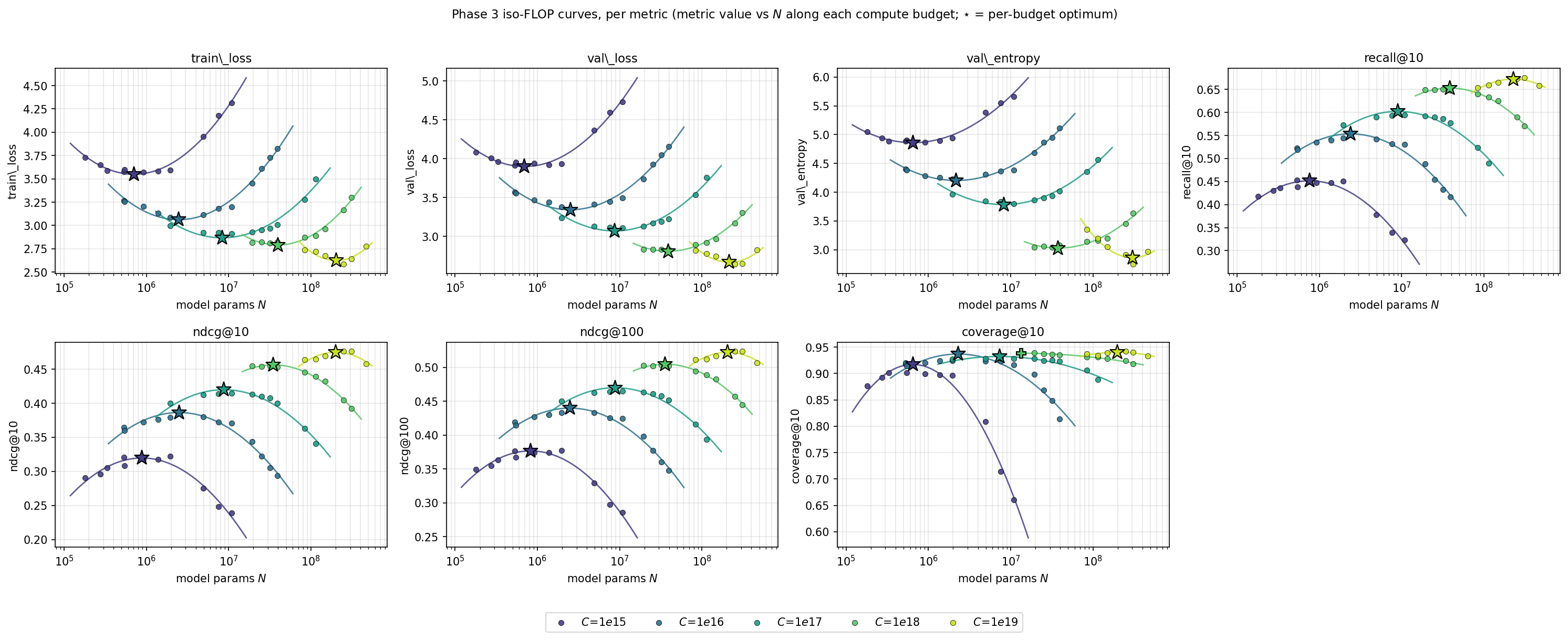
Now the Chinchilla question: with a fixed compute budget, do you want a bigger model trained on less data, or a smaller model trained on more? We trained dozens of models along iso-FLOP curves—lines of constant compute—at five budgets, and read off the winner at each (the stars back in ).

For language models, the compute-optimal ratio is about 20 tokens per parameter. Behavioral models look very different at small scale, and then converge:

D/N:   344  →  265  →  222  →  110  →  36

(data-to-parameter ratio at \(C = 10^{15},\,10^{16},\,10^{17},\,10^{18},\,10^{19}\) FLOPs)

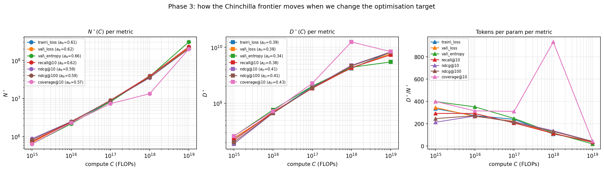
At small budgets, behavioral models want to be data-heavy: nearly an order of magnitude more data per parameter than a language model. But as compute grows, the ratio falls steadily toward the familiar Chinchilla regime. By \(10^{19}\) FLOPs we're within about \(2\times\) of the text-LM rule of thumb. The fitted law is

meaning the optimal recipe is moderately parameter-hungry as you scale up. shows the implied frontiers: optimal model size, optimal data, and the falling data/parameter ratio.

Batch size is usually treated as a boring engineering detail. In a scaling recipe, it's actually a tradeoff: a bigger batch is more hardware-efficient, but past a certain point each extra example stops buying proportional progress. That turning point is the critical batch size.

We measured how many updates it takes to reach a target quality at batch sizes from 64 to 2048, and fit the standard critical-batch model. Here's the twist: the knee depends on what you measure ().

• Validation loss and recall@10 share a knee near \(B \approx 570\).
• Top-weighted ranking metrics (NDCG@10, MRR@10) saturate much earlier, around \(B \approx 200\text{–}275\).
• Predictive entropy never plateaus in our range at all.

The intuition is simple: a metric that's only weakly sensitive to the loss in the operating region stops improving sooner, so its knee comes earlier. For throughput-limited production training, we recommend the largest batch we could run efficiently on a single node, \(B \approx 2048\)—just past the loss knee, where hardware efficiency wins.

Here's a quirk specific to behavioral models. To predict the next event, the model is trained to score the true next item higher than a set of negatives—plausible wrong answers. With a frozen, cached embedder, you can afford to throw many more negatives into the mix. So how many negatives \(K\) is best?

The useful range is broad but not arbitrary. Across budgets, the sweet spot for most metrics sits in the low hundreds of thousands (). But the story changes at the top end. At our largest budget, \(10^{19}\) FLOPs, every metric was still improving at the largest \(K\) we trained (2 million). At that point the bottleneck stops being compute and becomes plain memory: storing all those candidate scores. Negative sampling flips from a compute-allocation problem into a memory-engineering problem.

The practical rule: use \(K\) in the low hundreds of thousands when memory isn't binding, cap near \(10^6\) around \(10^{18}\) FLOPs, and treat anything beyond \(10^{19}\) as a memory problem to be solved with candidate sharding or checkpointing.

Step back and a single theme connects all four knobs. The model is trained on one thing—a sampled cross-entropy loss—but the deployed system is judged on another: how well it ranks items from the full catalogue. Those two quantities are usually correlated, but they don't always agree on which batch size, which architecture, or which negative count to ship.

Within a single training stage, the metrics look almost interchangeable—loss, perplexity, entropy, and the ranking metrics are correlated above 0.94 (). That makes it tempting to optimize loss and assume ranking follows. It mostly does. But "mostly" hides exactly the decisions a practitioner cares about.

The cleanest example is negative sampling after the embedder is frozen. The correlation between validation loss and recall@10 actually flips sign with compute: at \(10^{15}\) FLOPs the two are misaligned, while by \(10^{18}\) they agree perfectly (). The reason is mechanical—when you train against sampled negatives without correcting for how they were sampled, the model learns a popularity-biased ranking. Add enough negatives and that bias washes out, realigning loss with ranking. But until then, optimizing the training loss can quietly hurt the metric you actually serve.

One more practical wrinkle: cheap "batch-local" loss—measured against only the items in a validation batch—is a poor stand-in for true full-catalogue loss. But batch-local ranking metrics remain a reasonable proxy for comparing architectures. So if you're using a quick eval to pick a model, prefer ranking metrics over loss.

If you're already training the now-standard event-embedder → transformer stack, here's the distilled guidance. The most robust advice isn't any single number—it's the order of decisions: pick your deployment metric first, then set everything else.

One honest negative result worth flagging: we tried Maximal Update Parameterization (μP), which promises learning-rate transfer across model sizes. It delivered on transfer, but our plain truncated-normal initialization reached strictly lower training loss at every scale. So we kept the default and paid for a small per-phase learning-rate sweep instead.

Behavioral foundation models need their own scaling laws, and they don't simply inherit the language-model rules. Four things stand out:

1. Keep the embedder tiny (~2%). The part that understands products should be small; spend capacity on the part that understands people.
2. Start data-hungry, end Chinchilla-like. Behavioral models want lots of data per parameter at small scale, converging toward the text-LM ratio as you grow.
3. Batch size and negatives have wide but real sweet spots—and at the largest budgets, negative sampling becomes a memory problem, not a compute problem.
4. The metric is part of the scaling law. Decide what you're optimizing for before you tune anything, because the training loss is not always a faithful proxy for the ranking quality you deploy.

If you'd like the full derivations, fits, and appendices, read the complete paper. And if you want the broader story of why we train on actions in the first place, start with Large Behavioral Models.

• [1] Kaplan, J. et al. (2020). Scaling Laws for Neural Language Models. arXiv:2001.08361.
• [2] Hoffmann, J. et al. (2022). Training Compute-Optimal Large Language Models (Chinchilla). arXiv:2203.15556.
• [3] McCandlish, S. et al. (2018). An Empirical Model of Large-Batch Training. arXiv:1812.06162.
• [4] Yang, G. & Hu, E. (2021). Tensor Programs V: Tuning Large Neural Networks via Zero-Shot Hyperparameter Transfer (μP). arXiv:2203.03466.
• [5] Large Behavioral Models: A Foundation Model Paradigm for Human Actions. Unbox AI Blog, 2026.
• [6] A Foundation Model for Consumption, Transactions, and Actions: The Inception of BehaviorGPT. Unbox AI Blog, 2025.

@article{unbox2026scaling,
  author  = {Rickard {Br{\"u}el Gabrielsson}},
  title   = {Scaling Laws for Behavioral Foundation Models over User Event Sequences},
  journal = {Unbox AI Blog},
  year    = {2026},
  month   = jun,
  url     = {https://research.unboxai.com/scaling-laws-for-behavioral-foundation-models.html},
}